Navigation is a central element in almost any game. Understanding how players navigate through the virtual environment can offer valuable insights for game and level designers to build a robust and polished virtual environment. However, movement data is complex as it unfolds in space and time and visualizing trajectories individually very soon reaches its limit due to visual clutter and overplotting. Aggregation and simplification are two ways to reduce the complexity of data and the resulting visualization.
In this post I briefly introduce the concept of semantic trajectories1 for games user research and show how they can be visualized using transition diagrams. Semantic trajectories augment geospatial trajectories with semantic information and in doing so can be used to abstract from the raw position data, by viewing trajectories as a sequence of locations of interest. Assume you tell someone about a sightseeing tour in Barcelona, then you would likely focus on the sites and attractions you have visited rather than on the fine details of how you went from one location to another (unless perhaps something exciting had happened along the way). As such the tour is expressed by a sequence of points of interest.
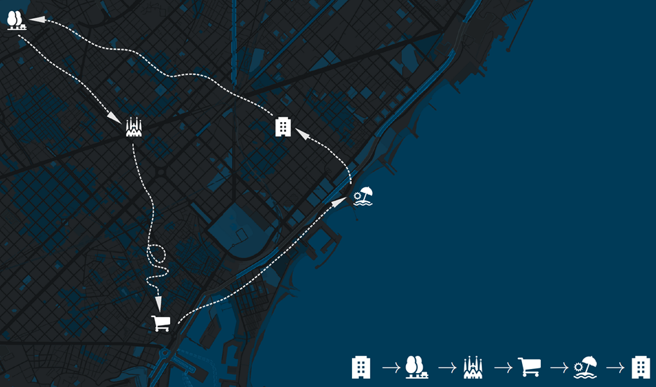
The idea behind is that often the exact routes are not necessary to comprehend the movement and the sequence of visited sites alone can offer already valuable insights. That also applies to games where the exact coordinates of player paths are not always necessary for understanding movement patterns (e.g., whether a player moved along the left or right side of a corridor) and the order in which certain locations are visited is sufficient.
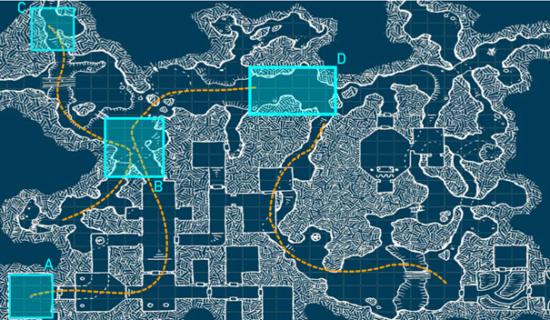
To derive semantic trajectories the raw trajectories positions can be compared with pre-defined areas of interest, as illustrated in the figure below.
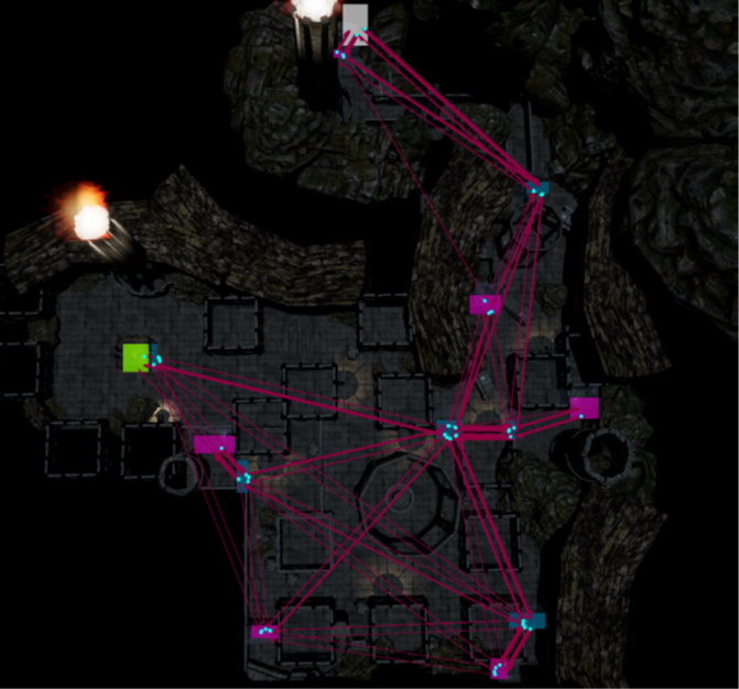
Once converted into sequences, transitions between areas can be visualized using, for instance, transition diagrams. Transition diagrams are used in many domains and come in different shapes but they have in common that they show the transitions between certain states (in our case the areas of interest). In the image below colored rectangles show the areas of interest while arrows show the transitions between areas. The thickness of the arrow can be used to indicate the amount of transitions. This way the resulting visualization is visually cleaner than when visualizing many individual raw trajectories.
On a side note, as semantic trajectories are (string) sequences, the similarity between semantic trajectories can be calculated with similarity measures such as longest common subsequence2 or Levenshtein distance3 which then, in turn, allows to apply clustering such as hierarchical clustering and identify outliers and common movement patterns.
Summary
In short, semantic trajectories allow to abstract from the complexity of raw trajectories by converting them into a sequence of locations. This allows to simplify the visualization and to establish the similarity between them more easily. Transition diagrams can be used to visualize them which reduces clutter and overplotting compared to visualizing the individual raw trajectories. This can help to identifier common movement patterns, outliers, and the frequency of visits of certain locations.
This blog post is based on the following publication: Schertler, R., Kriglstein, S., & Wallner, G. (2019). User Guided Movement Analysis in Games using Semantic Trajectories. In Proceedings of the Annual Symposium on Computer-Human Interaction in Play (pp. 613-623) (bibtex).
1 Parent, C., Spaccapietra, S., Renso, C., Andrienko, G., Andrienko, N., Bogorny, V., … & Yan, Z. (2013). Semantic trajectories modeling and analysis. ACM Computing Surveys (CSUR), 45(4), 1-32.
2 Hirschberg, D. S. (1977). Algorithms for the longest common subsequence problem. Journal of the ACM (JACM), 24(4), 664-675.
3 Wikipedia (2023). Levenshtein distance. https://en.wikipedia.org/wiki/Levenshtein_distance (Accessed: September 19, 2023)